Introduction to Wireless Links for Digital Communications
Part 2: Antennas
Daniel M. Dobkin
(revised December 2012)
Table of Contents:
The Ideal Dipole
Radiation Patterns
Some Common Antennas
The Ideal Dipole
Recall from our quick introduction in part 1 that all currents radiate. However, most currents cancel: if a current goes one way, a nearby current goes the other way to take the charge back so that it doesn't accumulate somewhere. The effects of such currents will often cancel out when viewed from far away. An antenna is a device whose purpose is to arrange currents so that their effects don't cancel at long distances, at least for some frequency range.
To see how this might work, we can examine a very simple example: the ideal dipole. This is an antenna consisting of a short length of thin wire (where 'short' is defined as much shorter than the wavelength of the radiation in question, and 'thin' is much smaller than 'short'). We have shown little caps on the ends to provide a place where the charge that flows through the wire can accumulate, since it has to go somewhere; the exact shape of the caps doesn't matter much as long as they're small compared to the length of the wire.
In order to keep things as simple as possible, we'll ignore the need for any generator of this current flow. How does the little bit of current that flows in the antenna affect distant objects? To find out, let's place a similar ideal-dipole antenna at some distance from our transmit antenna and use it as a receiver. Then we can formulate our question as: what voltage is induced in the receiving antenna when a current flows in the transmitting antenna? Again for maximum simplicity, we'll only consider the case where the receiver is located at a distance long compared to the wavelength and to the antenna side d, and at the same elevation as the transmitting antenna. In this case, the vector potential integral is very simple (just the product of the current Io and the length d of the dipole, divided by the distance, which is constant and can be pulled out of the integrand). The electric potential is zero, because for large r the distance to the top and bottom of the dipole is identical, but the charges there are opposite. The voltage induced in the receiving antenna is proportional to the line integral of the potential along the antenna; in this case, that's just the product of the vector potential and the receiving antenna length (again taken to be d). Note that we re-express the voltage in terms of the impedance of free space, Z0 = 377 ohms, so that the induced voltage has the form of the product of the transmitting antenna current and a resistance, multiplied by the ratio of the antenna height to the wavelength, and again by the ratio of the antenna height to the distance between the antennas.
We find that the induced voltage is inversely proportional to the distance, directly proportional to the peak current, and proportional to the square of the dipole length. To put some numbers in, imagine that the peak current is 1 amp, the frequency is 2.45 GHz (so one wavelength is about 12.2 cm), the dipoles are 1 cm long, and the separation between dipoles is 100 meters. We then find that the peak voltage induced on the receiving antenna is about 15 mV.
It isn't obvious from what we've derived so far, but it can be shown that the equivalent radiation resistance of this antenna is around 5 ohms. That means the transmitted power was about 2.6 W and the received power is about 5.6 microwatts, assuming a matched generator and load. This doesn't seem like much power, but by reference to the previous section we see that the received power of around -23 dBm is still huge compared to the thermal noise (around -90 to -100 dBm for a high-rate, MHz-bandwidth signal such as a local-area network); a well-designed receiver ought to have no trouble extracting the modulation from this received power.
We have shown the calculation only for the case where the two antennas are horizontally oriented with respect to one another. It is possible, though more laborious, to use the same approach for the case where the antennas are oriented along the vertical axis; in this situation, we obtain the interesting result that the electrostatic potential induced by the charges on the ends of the antenna is exactly enough to cancel the voltage due to the vector potential induced by the current: the dipole does not couple along its axis. A dipole is a directional antenna: most of the radiated power is directed in the horizontal plane.
Radiation Patterns
It is clearly somewhat inconvenient to perform this calculation for every conceivable pair of antennas in every geometry. Fortunately, we don't need to. It turns out that under fairly plausible assumptions, the received power at any antenna can be calculated if we know the directive gain of the transmitting and receiving antennas and the separation between them. (The use of the word 'gain' associated with antennas is an inevitable source of confusion. Antennas are passive devices and radiate at best as much power as you put into them. They can, however, put more of that power into one direction than another, resulting in an effective increase in received power -- 'gain' -- in the favored direction.)
To quantify this assertion, we need to find the relationship between the potential calculated above and the radiated power. By a simple heuristic argument we can show that this ought to be:
where P is the power radiated at distance r per unit cross-sectional area, and the subscript 'tr' denotes the part of the vector potential which is transverse to the observation vector r. The corresponding power for the ideal dipole is also shown, where the angle is defined with respect to the axis of the dipole. Also shown in the quantity U obtained by multiplying P by the square of the distance; U gives a measure of the angular distribution of the radiated power. U is known as the radiation intensity. A graphic depiction of U vs. angle is a radiation pattern for the antenna; such an image for an ideal dipole is shown below:
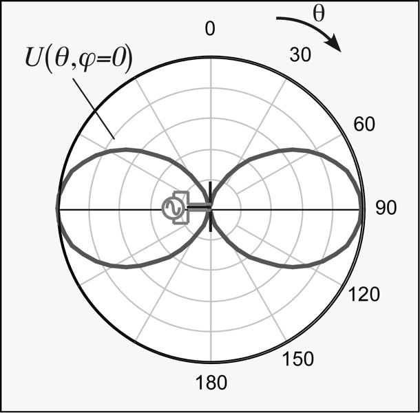
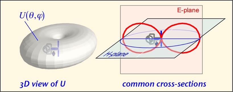
In this graphic, the distance of the black curve from the origin denotes the corresponding radiation intensity, normalized to the maximum value, for that value of inclination angle. Thus, the radiation intensity is zero along the axis of the dipole, and reaches its maximum at an angle of 90 degrees from the axis. This picture is known as an E-plane cross-section of the radiation pattern; a pseudo-three-dimensional view and two corresponding cross-sections are shown in the next image:
In most cases, the user of an antenna is interested in its performance in the direction where most of the radiated power is: the maximum directive gain or directivity. If the antenna is perfectly efficient (all the input power is radiated) this is numerically the same as the antenna power gain. These quantities are always normalized to the power radiated by the antenna averaged over all angles, so that they represent the excess power in a particular direction vs. an ideal isotropic antenna The maximum directive gain of an ideal dipole is D = 3/2 or 1.8 dBi (the terminology refers to dB of gain relative to an ideal -- and non-existent -- isotropic antenna).
In nearly all cases of practical interest, the properties of a receiving antenna are closely correlated to its behavior as a transmitter; thus, the same power gain can be used to characterize both transmission and reception. Therefore, we can find the received power of a link composed of a pair of antennas in terms of the transmit power, the wavelength, the distance between the antennas, and the gains of the antennas: the Friis equation --
The Friis equation provides us with the effects of antenna gains and path loss in the link budget calculation we performed in part I.
We can see that the power gain of the antennas used in a link is what affects the link performance. However, in practical use the antennas must get power from the generator and deliver it to the load. Like any other electrical system, antennas work best when their impedance is well-matched to that of the generator or load. Most radio systems use a characteristic impedance of 50 ohms; thus the easiest antennas to use are those whose electrical impedance is close to 50 ohms. Antenna selection is also influenced by convenience, cost, robustness under mechanical stress (portable devices) or wind, rain, sun, and snow (outdoor installations), and esthetics. In handheld devices, safety is also important: antennas and systems are designed to reduce the amount of power coupled into a user’s head when a phone handset is held near the ear.
Survey of Common Antennas
Here we examine the working principles and characteristics of a few common antenna types.
One of the simplest and most frequency-used antennas is the half-wave dipole. This is simple a pair of wires, cumulatively about a half of the wavelength of the relevant radiation in length, driven at the center by an imposed voltage. To a good approximation, the current along the dipole can be taken to be sinusoidal: it is maximized at the center and goes to zero at the ends (where, after all, there is no place for it to go).
The potential can then be obtained by integrating over the current distribution. The square of the transverse part provides the radiation intensity and the antenna pattern. The resulting expression is a bit more complex than that for the ideal dipole, but qualitatively similar: most radiation is in the horizontal plane through the antenna feed, and the radiated power goes to zero along the axis. The directivity is a bit higher than that of an ideal dipole: D is about 1.64 or 2.2 dBi. Half-wave dipoles are easy to build, and for typical wire sizes their impedance is nearly resistive and just under 70 ohms; thus a reasonable match is obtained to a 50 ohm cable with no particular precautions. However, a half-wave dipole is a balanced antenna, and should be driven by a balanced signal (in which the top and bottom voltages are equal and opposite with respect to ground). A coaxial cable is not a balanced signal source; a balanced-unbalanced transformer or balun should be used to convert between the antenna and cable.
A closely related alternative is the quarter-wave monopole. In this case, the image of one wire in a conducting ground plane is used to provide the other half of a half-wave dipole. Monopoles are also easy to build, and since the monopole has a ground plane it doesn't require a balun to interface with a coaxial feed cable.
The electrical properties are similar to those of a half-wave dipole, but (for an infinite ground plane) there is no radiation below the ground plane, so the directivity of the antenna is increased by a factor of 2 (3 dB). Real finite ground planes allow some radiation to the lower hemisphere.
A directional antenna that is very simple to construct at microwave frequencies (for example, for 2.4-2.5 GHz ISM band applications like wireless LANs) is the waveguide antenna or cantenna. A cantenna is just a waveguide that supports a propagating mode at the frequency of interest, open at one end.
Any closed conducting shape, such as a rectangular prism, tall cylinder, or ellipsoid, can act as a waveguide, allowing unattenuated propagation of electromagnetic waves along its length. To propagate in this fashion, the wave must meet the boundary conditions imposed by the metallic walls: these are approximately equivalent to forcing the potential to zero at the metal surface. A very low frequency wave cannot manage such a feat: the wavelength must be roughly comparable to the size of the waveguide to allow the potential to reach zero at opposing ends of a diameter. Thus, any waveguide has a cutoff frequency below which waves are exponentially attenuated in amplitude as they move into the guide.
Above the cutoff frequency, the phase velocity of the wave varies rather rapidly with frequency, so that in a long guide some dispersion would result. (That is, waves of slightly differing frequencies move at a different rate, resulting in distortion of modulated signals. For those in the San Francisco Bay Area, a lovely demonstration of this effect for sound waves can be heard at the Exploratorium in San Francisco.) Dispersion is of modest concern for a typical cantenna, which is fairly short and gives little room for distortion to take place. Thus, a cantenna must be large enough for one mode at the desired frequency to propagate, and preferably not so large that other modes (shapes of the potential) can also propagate. These constraints set a lower and upper limit for the diameter of a cylindrical waveguide. For a cylinder, the lowest-frequency propagating mode has a wavelength about 3.4*(radius of the cylinder), and the next-lowest mode is at about 2.6*(radius). For 2.4 GHz, this means the cantenna radius should be around 7-9 cm. It's better to miss high, since a second propagating mode has only a modest effect on performance, whereas if the desired frequency is too low, the fundamental will not penetrate the waveguide.
A simple solution to getting the wave in and out is to employ a quarter-wave monopole, using the cylinder as the ground plane. The monopole electrical characteristics are fairly similar to those obtained from a flat ground plane. The best place to locate the antenna is a quarter of the guide wavelength from the (reflecting) end of the can. In this arrangement, the image of the dipole formed by the reflector is a half-wave distant. Since the image current is the negative of the real current, and a half-wave distance inverts the sign of the potential, the reflected wave will be in phase with the direct wave from the antenna, and the two add to create an enhanced transmitted field. Note the spacing must be in terms of the guide wavelength, which is in general somewhat longer than the wavelength in open space.
The directive gain in the cantenna comes from the increased exit aperture. A fair approximation to the directivity can be obtained simply by dividing the physical aperture (the area of the can exit) by the aperture of an ideal isotropic antenna, which is the square of the wavelength divided by 4π. An example for the smallest allowed cylindrical antenna gives:
More directive gain can be obtained by flaring the end of the waveguide to a larger aperture, though the transition needs to be sufficiently gradual to minimize disturbance to the propagating wave: in this fashion one obtains a horn antenna.
Punch a Hole, Name an Antenna
The examples above are just a tiny start on the absurdly long list of antenna types. Any structure that can create unbalanced currents can be useful in the right circumstances. Huge parabolic reflectors can be used to achieve directive gain measured in tens of dB’s. Metal plates with slots can be used to make antennas with multiple resonances at carefully-chosen frequencies (like the bands used for cellular communications), while not being too bothered by the presences of people’s hands a centimeter away. Arrays of antennas with differing relative phase can adaptively direct a beam or adaptively select an incoming signal.
For a more detailed discussion of these topics, see Dan's (now somewhat dated) book, RF Engineering for Wireless Networks, Elsevier 2004. If you really want to take the plunge, get Antenna Design (Third Edition), C. Balanis, Wiley 2005; the hardback is also useful for upper-body exercises.